Units

The SatAndLight software makes use of a uniform set of units. As a result, the choice of units is not always adapted to the quantity it measures. However, it is preferable to work this way to avoid multiple unit conversion. The user will have to make sure the correct units are used for any quantity provided to the software. The following table lists the units used in SatAndLight.

Quantity	Unit
Length	\(\mathrm{mm}\)
Time	\(\mathrm{ms}\)
Energy	\(\mathrm{keV}\)
Angle	\(\mathrm{rad}\)

Coordinates

Two reference frames are used in SatAndLight:

The satellite reference frame, \({\cal{R}}\), with a system of coordinates \((x,y,z)\).
The Earth reference frame, \({\cal{R'}}\), with a system of coordinates \((x',y',z')\).

All quantities associated to the Earth reference frame are primed while those associated to the satellite reference frame are not. A three-dimensional rotation is used to change the reference frame and is described by the Rotation class.

Earth

The Earth reference frame, \({\cal{R'}}\), is given celestial coordinates. The Earth celestial coordinate system is \((x',y',z')\) and its origin is located at the center of the Earth. The \(z'\) axis is the rotation axis of the Earth and points to the North pole. The \(x'y'\) plane is the equatorial plane, and the \(x'\) axis points to the vernal equinox.

Earth reference frame and celestial coordinates.

All quantities measured in \({\cal{R'}}\) are primed quantities. Spherical coordinates are used to set a direction in the sky:

\(\theta'\) is the angle between the \(z'\) axis and the direction of interest: \(0\le\theta'\le\pi\).
\(\varphi'\) is the angle between the \(x'\) axis and the projection of the direction of interest on the \(x'y'\) plane: \(0\le\varphi'<2\pi\).

Alternatively, the right-ascension ( \(=\varphi'\)) and the declination ( \(=\pi/2-\theta'\)) can be used to set a direction in the sky.

All angles are measured in \(\mathrm{rad}\).

System

A system refers to a satellite or a part of a satellite. The system reference frame, \({\cal{R}}\), is given system of coordinates \((x,y,z)\). By convention, the \(x\) axis is used as the pointing axis of instruments, like telescopes.

Geometrical definitions. The rotation to change the system of coordinates is given by the Euler angles and is represented in green.

The system reference frame is placed in the Earth reference frame and a three-dimensional rotation is used to change reference frames (see the Rotation class). The rotation is performed using Euler angles \(\alpha,\beta,\gamma\).

A direction of interest in the sky is measured using spherical angles:

\(\theta\) is the angle between the \(x\) axis and the direction of interest: \(0\le\theta\le\pi\).
\(\varphi\) is the angle between the \(y\) axis and the projection of the direction of interest on the \(yz\) plane: \(0\le\varphi<2\pi\).

Note: This is not standard spherical coordinates as the \(x\) axis is the "vertical" axis.

System reference frame and associated coordinates.

Astrophysical source

SatAndLight is designed to simulate various astrophysical sources (see the Source class). Once parameterized, a source can produce astro-particles which can interact with satellite instruments. A source is characterized by:

a position in the sky: this is measured by 2 angles
an area in the sky: this is modeled by a cone centered in the source position
a particle emission: this is described by a Flux.

Position

The position of a source in the sky is measured by 2 angles. The Earth reference frame is primarily used and sherical coordinates are used.

Flux

An astrophysical source is characterized by a particle flux which measures the particle energy density, \(\frac{dN}{dE}\), crossing a unit surface per unit time:

\[ {\cal{F}}(E,t)=\frac{d^4N}{dSdtdE}(E,t). \]

The flux is a function of time and energy and is measured in \([\mathrm{keV}^{-1}\mathrm{ms}^{-1}\mathrm{mm}^{-2}]\). By convention the flux is measured "on-axis", meaning that the particle direction is perpendicular to the surface. Therefore the flux must be corrected by a \(\cos\theta\) factor if the incoming direction is angled.

Particle flux definition.

Warning: By convention, we call particle flux, or simply flux, the particle energy density flux \({\cal{F}}(E,t)\).

Rate

The particle rate measures the particle energy density, \(\frac{dN}{dE}\), per unit time. It can be obtained by integrating the particle flux over the surface of interest:

\[ {\cal{R}}(E,t)=\frac{d^2N}{dtdE}(E,t)=\iint_S{\cal{F}}(E,t)dS=\iint_S\frac{d^4N}{dSdtdE}(E,t)dS. \]

The rate is a function of time and energy and is measured in \([\mathrm{keV}^{-1}\mathrm{ms}^{-1}]\).

SpecTime

The particle emission from a source is usually discribed by 2 quantities:

A light curve which measures the rate of particles as a function of time: \({\cal{L}}(t)=\frac{dN}{dt}(t)=\int_0^{+\infty}{{\cal{R}}(E,t)dE}\). It is obtained by integrating the particle rate over all possible energies.
An energy spectrum which measures the particle flux, averaged over a time \(T\), as a function of energy: \({\cal{S}}(E)=\frac{1}{T}\int_0^T{{\cal{F}}(E,t)dt}\)

For SatAndLight, the SpecTime class is used to describe both the particle flux, \({\cal{F}}(E,t)\), and the particle rate, \({\cal{R}}(E,t)\). These functions are described by 2-dimensional histograms (TH2D in ROOT), where the x-axis is binned in time and the y-axis is binned in energy. Each bin contains the particle flux \({\cal{F}}(E,t)\) (or rate) measured at the center of the bin. This object is called a SpecTime object.

See also: snl-spectime.cc which is an application used to produced SpecTime objects.

[ADD AN EXAMPLE]

Telescope

Acceptance

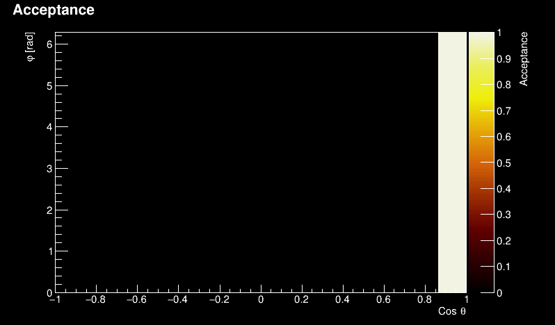
A telescope is given an acceptance function which measures the probability to detect an astro-particle given its incoming direction. The incoming direction is given by two angles, \(\theta\) and \(\varphi\), measured in the telescope reference frame. The acceptance function is defined as:

\[ A=A(\cos\theta,\varphi), \]

and

\[ 0\le A \le 1. \]

The acceptance function can be used to simulate the telescope field of view: \(A=1\) when \(\theta\) is smaller than the opening angle, \(A=0\) otherwise.
The acceptance can be used to simulate vignetting effects: \(A<1\) for edge values of \(\theta\).
Cosmic rays can be detected from many directions. Complex acceptance functions can be used to simulate the particle shielding in the satellite.

In SatAndLight, the acceptance function \(A(\cos\theta,\varphi)\) is formatted as a 2-dimensional histogram: ROOT TH2F. The x-axis is binned in \(-1 \le \cos\theta \le 1\) and the y-axis is bin in \(0 \le \varphi < 2\pi\).

For example, a telescope can be defined by an opening angle, say 60 degrees. In that case, photons can only be detected if the incoming direction is inside a cone such as \(\cos\theta>\cos(30)=0.866\). As a result, the acceptance object looks like:

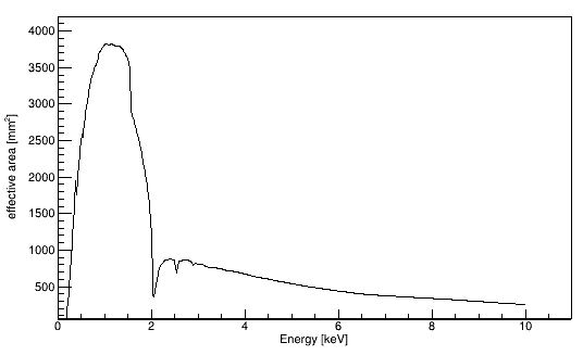
Photon acceptance for a telescope with a 60 degrees opening angle.

Effective area

The effective area measures the ability of a telescope to detect an incoming astro-particle (not just photons!) of a given energy. The telescope sensitive area (e.g. CCD) has a physical size. The greater is the physical size, the more astro-particles can be detected. Effectively, the sensitive area can be impacted by the optical property of the telescope (e.g. reflectivity) which can be a function of energy. The effective area, \(S(E)\), is used to measure the particle rate at the level of the telescope:

\[ {\cal{R}}(E,t)=\frac{d^2N}{dtdE}(E,t)=\iint_S{\cal{F}}(E,t)dS=S(E)\times {\cal{F}}(E,t). \]

In SatAndLight, the effective area is formatted as a ROOT TGraph. The x-axis masures the energy in \([\mathrm{keV}]\) and the y-axis measures the effective area in \([\mathrm{mm}^2]\).

Effective area for the MXT (SVOM satellite)

See also: snl-acceptance.cc to generate an acceptance object.

Warning: These are all on-axis quantities. A \(\cos\theta\) factor should be used to describe off-axis detections.

Note: In general, the effective area should also include a \(\theta\) dependence to describe effects like vignetting. This dependence is managed with the telescope acceptance.

Example to generate an effective area TGraph from an Ancillary Response File (ARF):

TFITSHDU *f = new TFITSHDU("./my_arf.arf");
f->Change(1);
TVectorD *energy = f->GetTabRealVectorColumn(0);
TVectorD *effarea = f->GetTabRealVectorColumn(2);
TGraph *graph = new TGraph();
for(int i=0; i<energy->GetNoElements(); i++){
  if(effarea->GetMatrixArray()[i]>=0.0)
    graph->SetPoint(graph->GetN(), energy->GetMatrixArray()[i], effarea->GetMatrixArray()[i]*100.0);
}
TFile *fout = new TFile("./effective_area.root", "recreate");
fout->cd();
graph->Write("effarea");
fout->Close();

Point spread function PSF.

The telescope point spread function, \({\cal{P}}={\cal{P}}(y,z,E)\), describes the telescope optical system. The optical system is assumed to be linear and the PSF can be seen as a probability density function used to deflect the photon hit position in the camera plane. For a point-like source, the resulting image is a specific pattern shaped according to the PSF distribution. First, the photon hit position is determined without optics, simply considering the telescope acceptance: \((y_0,z_0)\), in camera intrinsic coordinates. Then the final hit position is computed with the probability density \({\cal{P}}(y-y_0+1,z-z_0+1,E=E_{photon})\).

Internally, the PSF function must be limited in size. For spatial coordinates, we choose to have \(y\) and \(z\) running from 0 to 2 in intrinsic camera coordinates. Moreover, the optical axis must cross \(y=1\) and \(z=1\) for the PSF function. With such a configuration, it is possible to shift the PSF function from \(y,z=0\) to \(y,z=1\) and have a full camera plane coverage by the PSF function. The energy parameter is running from a minimum to a maximum value set by the user. Outside this ranges, photons are not transmitted to the camera plane.

Internally, the PSF is represented as a ROOT TH3F histogram. The X (resp. Y) histogram axis matches the Y (resp. Z) axis of the camera plane. The Z axis is binned in energy. Each bin is given the probability density for \((y,z,E)\) measured at the center of the bin. The normalization of the PSF does not matter as it is internally normalized when computing probabilities. The \(y\) and \(z\) coordinates must run from 0 to 2 to allow for every possible shifts over the camera plane, assuming the PSF peak is positioned at \((y=1,z=1)\).

Note

Assumptions made for the PSF:

the PSF is shift-invariant.
The PSF spatial coordinates run from 0 to 2.
The telescope optical axis is centred on \(y=1\) and \(z=1\).

See also: snl-psf.cc to generate a PSF object.

Table of Contents